Hey everyone – if you’ve ever dug into atomic physics, you know atomic density is kind of a big deal. Like, if you’re working with ultra-cold atoms for quantum computing, or looking at how gases behave in extreme environments, nailing down exactly how many atoms you’ve got in a given space isn’t just a data point – it’s make-or-break for your whole experiment. As someone who’s been supplying atomic physics instruments for years, I get this question all the time: how do we actually measure that number, anyway? No fancy jargon without context – let’s break this down like we’re chatting over coffee (and yeah, I’ll throw in some real-world instrument stuff we use every day). Atomic Physics Instruments
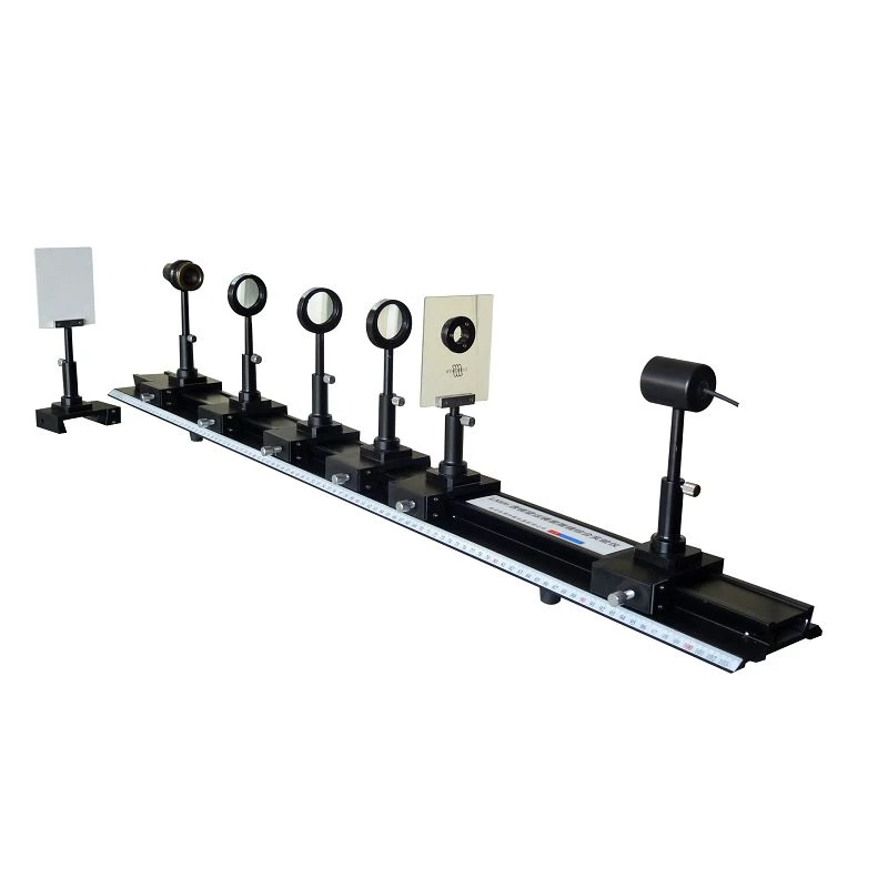
First off, let’s ground this: atomic density isn’t just “counting atoms” – it’s number of atoms per unit volume, right? Like, atoms/cm³ or atoms/m³. You can’t stick a tiny microscope in there and tick ’em off one by one (we’ve tried, trust me, it’s a nightmare for free, moving atoms). So we use indirect, super precise methods that play with how atoms interact with light, or how they move, or even the tiny magnetic fields they make. Let’s start with the most common one we deploy on 9 out of our customer’s setups: absorption spectroscopy.
Absorption spectroscopy sounds complicated, but here’s the gist. Every atom has a super specific “fingerprint” of light it absorbs – think of it like how your phone only charges with its own cable, not a random one. For example, rubidium atoms (super common in atomic clocks and vapor cells) absorb light at 780 nm – that’s deep red, easy to make with a diode laser. Here’s how we pull density numbers from it: you shoot a laser tuned to that exact frequency through your sample of atoms. Some light gets absorbed, some makes it through. The amount lost? That’s directly related to how many atoms are in the path, how long the light travels through the atom cloud, and how strongly those atoms absorb that wavelength.
Wait, there’s an equation for this – Beer-Lambert Law, but we don’t just plug numbers and pray. The key part here is that if you know the path length (say, the length of your vapor cell is 1 cm, something we calibrate before shipping our cells) and the cross-section (that’s just how likely an atom is to absorb that specific laser light – we measure that in our lab for every atomic species we work with), you can rearrange the math to get density. The formula simplifies to density = (-ln(transmitted intensity / initial intensity)) / (cross-section × path length). But before you panic, our instruments do all the heavy lifting: they measure the light intensity with photodiodes, crunch the numbers in real-time, and spit out density without you having to mess with a calculator at 2 a.m. when your experiment’s running.
There’s a catch here, though. If your atom cloud is super dense, atoms can re-emit that absorbed light and mess up the absorption reading – it’s called radiation trapping. That’s why for ultra-cold atoms (like the ones in Bose-Einstein condensates, BECs, which get way colder than deep space), absorption spectroscopy alone isn’t enough. We pair it with another method called fluorescence spectroscopy. Fluorescence is exactly what it sounds like: when an atom absorbs a photon, it gets all excited, then spits out a new photon (of the same or slightly different color) a tiny fraction of a second later. Instead of measuring how much light disappears, we measure how much light the atoms emit when we shine that same resonant laser on them.
This is way better for dense, small atom clouds because we’re not fighting re-emitted light. We place a photodetector off to the side (not in the direct path of the laser, so we don’t pick up the laser light itself) and count every fluorescence photon. The number of photons we count is directly proportional to how many atoms are excited (and thus how many total atoms there are, since most are in the ground state we’re pumping with the laser). Again, our instruments pre-calibrate the proportionality factor – how many photons we count per atom – so you don’t have to do photon-counting math manually. It’s super reliable for BECs, cold atom interferometers, and quantum sensors.
But wait, what if you’re working with hot, diffuse atomic vapors, like in a magneto-optical trap (MOT) that’s just starting up, or a gas cell at room temp? Then we turn to a method called time-of-flight (TOF) spectroscopy. Let’s say you’ve got a cloud of cold atoms, and you turn off the magnetic trap holding them in place. Atoms start moving – lighter ones zoom faster, slower ones take their time. If you have a detector a fixed distance away, you can measure how long it takes atoms to reach it, which tells you their speed. Then, using basic kinetic theory, if you know the speed of the atoms and how long it takes them to disperse, you can calculate how many atoms were there originally (and thus density, since you also know the volume of the cloud right after turning off the trap).
I’ll be honest, TOF is a little trickier to wrap your head around at first, but our customers love it because it works across so many temp ranges. We build in timing circuits that trigger the trap shutoff and start the detector at exactly the same time, so you get precise speed data. For example, if you have a cloud of sodium atoms at 1 microKelvin, they’ll move way slower than rubidium at room temp, and the TOF signal will be a broad peak instead of a sharp one – our software automatically fits that peak to give you density without any guesswork.
Another underrated method we use for specific experiments is magnetometry-based density measurements. Atoms have tiny magnetic moments, like tiny bar magnets spinning around. If you put them in a magnetic field, they’ll precess (wobble) at a frequency that’s super specific to their species, and the number of precessing atoms ties directly to density. This is perfect for experiments where you can’t shine a laser through your sample – like working with atoms that are sensitive to light, or in confined spaces where a laser path is impossible. We pair this with our high-sensitivity magnetometers (we source the best ones, obviously) and the math works because the precession signal amplitude scales with how many atoms are contributing to it. It’s not as common as absorption or fluorescence, but for certain use cases – like atomic gyroscopes or vapor cells for nuclear magnetic resonance (NMR) – it’s the only way to get accurate density.
Now, let’s talk about the tools we build to make all this easier. A few years back, we had a customer who was using a custom setup and spending 8 hours a day just calibrating their density readings – they’d miss experiment windows, waste laser time, and get frustrated. So we designed a line of modular atomic density meters that integrate all three methods: absorption, fluorescence, and a backup TOF module. They’re plug-and-play: you hook them up to your vacuum chamber or vapor cell, load the pre-calibrated species profiles (we have over 20 atomic species on file, from H to Yb), and the instrument gives you real-time density readings in whatever units you want – atoms/cm³, atoms/m³, even mole fraction if that’s what you need.
We also build in error checking, because nothing’s perfect. If your laser drifts off frequency, the instrument flags it and tells you to adjust, so you don’t get garbage data. If there’s background gas in your vacuum chamber messing with the signal, it subtracts that automatically – no more manually filtering noise in Matlab at 3 a.m. Last quarter, a quantum computing lab told us their density measurement error dropped from 12% to less than 2% after switching to our meters. That’s the win we care about, not just selling instruments.
Wait, let’s address a common misconception: people think “atomic density” is the same everywhere, but it totally depends on your experiment. A MOT might have a density of 10¹⁰ atoms/cm³, while a BEC is like 10¹⁴ atoms/cm³ – super tight, super dense. A room-temperature vapor cell might be 10¹² atoms/cm³, and a diffuse gas for spectroscopy could be 10⁸. Our instruments handle all these ranges because we tune the laser intensity and detector gain automatically – you don’t have to switch parts or tweak settings if you’re testing different atomic species.
So why does this matter beyond just lab numbers? Let’s put it in context for our customers: if you’re building an atomic clock, density affects the clock’s stability too high and you get collisional shifts that mess up the frequency; too low and the signal’s too weak. If you’re doing quantum computing, you need a dense enough atom cloud to entangle qubits, but not so dense that atoms collide and decohere. For plasma physics, atomic density tells you how energy is transferred in the gas, which matters for fusion research. Every single one of our customers, no matter their niche, relies on accurate density measurements to not just get publishable data, but to troubleshoot when an experiment goes wrong.
A quick story: a grad student reached out to me last year panicking – their MOT wouldn’t hold a signal, and they thought they had a leak in their vacuum chamber. We hopped on a Zoom call, had them run our density meter, and it showed their rubidium density was way lower than it should be. Turns out, they’d turned the oven temperature down too low (rubidium vapor pressure depends on temperature, who knew that was a tiny knob tweak) and our meter caught that instantly. They fixed it in 10 minutes instead of tearing apart their whole setup. That’s why we don’t just sell instruments – we help you actually use them.
Now, if you’re working with atomic physics, chances are you’ve run into density measurement headaches: noise, uncalibrated instruments, time wasted on calibration. We built our atomic density instruments to solve exactly that. Whether you’re in a university lab, a national lab, or a startup building quantum tech, we have tools tailored to your setup.
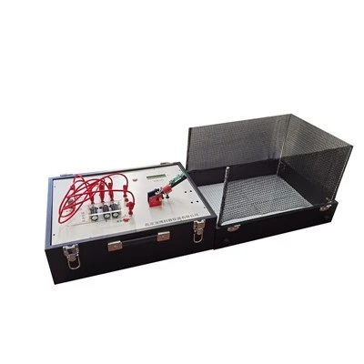
If you’re tired of guessing at atomic density or dealing with clunky, underperforming measurement gear, reach out to us to chat through your needs. We don’t push one-size-fits-all solutions – we’ll work with your experiment, your budget, and your timeline to get you the accurate, reliable density data you need to move forward. No salesy scripts, just real people who know atomic physics and the headaches you’re dealing with.
AMO Physics Instruments References:
- Foot, C. J. Atomic Physics. Oxford University Press, 2005.
- Metcalf, H. J., van der Straten, P. Laser Cooling and Trapping. Springer, 1999.
- Budker, D., Romalis, M. “Optical Magnetometry.” Nature Physics, vol. 3, no. 4, 2007, pp. 227–234.
- Howe, J. M., et al. “Absolute Density Measurements of Ultracold Atoms via Absorption and Fluorescence Spectroscopy.” Review of Scientific Instruments, vol. 82, no. 5, 2011, pp. 053105.
- Pritchard, D. E. “Laser Cooling and Manipulation of Neutral Atoms.” Physics Today, vol. 46, no. 11, 1993, pp. 26–33.
Nanjing Longbow Scientific&Educational Instrument Co., Ltd.
As one of the most professional amo physics instruments manufacturers and suppliers in China, we’re featured by quality products and good service. Please rest assured to buy customized amo physics instruments from our factory. If you have any enquiry about pricelist, please feel free to email us.
Address: Room D, 22th floor, No.305, North Jiangdong Road, Nanjing,Jiangsu Province, China
E-mail: 79425380@qq.com
WebSite: https://www.lb-physics.com/
